Shared Actors Need Not Share Critics

Effects of Value Mismatch in Parallel Reinforcement Learning

Zhenya Liu^1*, Yang Meng¹, Zhuokai Zhao¹, Xuefeng Liu^2† & Yuxin Chen^1†*

¹University of Chicago · ²University of Florida

^†Equal supervision. ^*Corresponding authors.

TL;DR

Problem

The same behavior may be desirable across environments even when their value targets differ. A shared critic averages those targets and miscenters the sampled advantages used for learning.

Method

Condition only the critic on a logged environment index, while keeping the actor, sampling protocol, and PPO pipeline shared.

Strongest result

On held-out Procgen levels, a multihead critic improves aggregate normalized return by 40.8% across 16 games (600 unseen levels per game). On BipedalWalker, it raises final mean return from 90.7 to 190.4 on 100 unseen terrains.

arXiv alphaXiv

@misc{liu2026sharedactors,
  title  = {Shared Actors Need Not Share Critics: Effects of Value Mismatch in Parallel Reinforcement Learning},
  author = {Liu, Zhenya and Meng, Yang and Zhao, Zhuokai and Liu, Xuefeng and Chen, Yuxin},
  year   = {2026},
  eprint = {2608.26481},
  archivePrefix = {arXiv},
  primaryClass = {cs.LG},
  url    = {https://arxiv.org/abs/2608.26481}
}

GitHub

Motivation

From sampled policy updates to value mismatch

Policy gradient optimizes the expected return $J(\theta)=\mathbb E_{\tau\sim\pi_\theta}[G(\tau)]$ by updating a stochastic policy from sampled trajectories. A sampled update is proportional to $(G_t-B_t)\nabla_\theta\log\pi_\theta(a_t\mid s_t)$ . An action-independent baseline cancels from the expected gradient, but it still determines the sign and size of each realized step; that step changes the policy that generates the next sample.

Parallel reinforcement learning commonly pools rollouts from many environments to train one actor. This is natural when the same behavior is desirable across environments, even if their dynamics and returns differ.

The critic solves a different prediction problem: the correct value can depend on an environment identity that is hidden from the actor but logged during rollout collection. At its population target, a shared critic averages these distinct values and thereby shifts the sampled advantages within each environment.

What do these shifts do to the finite sample optimization path when the expected policy-gradient update agrees at the same policy?

(a)

Shared baseline

$q_E=q_H=\tfrac12$ in this illustration

$V_E^\pi(s)$ environment E target

$\bar V^\pi(s)$ one marginalized value

$V_H^\pi(s)$ environment H target

e_E^\pi(s)=V_E^\pi(s)-\bar V^\pi(s)>0

e_H^\pi(s)=V_H^\pi(s)-\bar V^\pi(s)<0

$B^{\mathrm{shared}}(s)=\bar V^\pi(s)=\tfrac12\!\left[V_E^\pi(s)+V_H^\pi(s)\right]$

(b)

Conditional baseline

the same two environment values

$B^{\mathrm{cond}}(s,E)=V_E^\pi(s)$ environment E centered

$B^{\mathrm{cond}}(s,H)=V_H^\pi(s)$ environment H centered

V_E^\pi(s)-B^{\mathrm{cond}}(s,E)=0

V_H^\pi(s)-B^{\mathrm{cond}}(s,H)=0

$B^{\mathrm{cond}}(s,z)=V_z^\pi(s)$

Paper preset: $\eta=2$ , 100 updates, 4,000 paired trajectories, $q(E)=q(H)=\tfrac12$ , and $\pi_0=(0.34,0.33,0.33)$ . Each cloud shows the sampled policy distribution; faint paths trace representative runs and the solid path traces the mean policy. Both panels reuse the same environment and action uniforms.

Value mismatch as a baseline shift. At the same critic input

s

, a critic without the environment identity predicts the marginalized value

\bar V^\pi(s)=\sum_z q_z^\pi(s)V_z^\pi(s)

. Its sampled advantage in environment

z

is shifted by

e_z^\pi(s)=V_z^\pi(s)-\bar V^\pi(s)

. Conditioning on

z

instead centers each environment at its own value target.

Theory

Same mean update. Different sampled paths.

The shared critic's value prediction is not necessarily noisy or poorly trained. Under squared error it is the best population prediction available without environment identity. The issue is how its systematic offset is allocated across realized environment–action samples.

Value mismatch identity

A^{\mathrm{shared}}_t=A^{\mathrm{cond}}_t+e_{Z_t}^{\pi_t}

with

e_z^\pi=V_z^{\pi}-\bar V^{\pi}

Population projection. Without environment identity, the squared-error optimum is $\bar V^\pi(s)=\mathbb E[G\mid S=s]=\sum_z q_z^\pi(s)V_z^\pi(s)$ . The shared critic's value prediction can therefore be statistically correct while remaining systematically miscentered within each environment.

Proposition 1 · why convergence first

A common destination and a rate for time averages

For finite deterministic bandits with a common strict optimal arm, the No baseline, Shared baseline, and Conditional baseline processes converge almost surely to the same arm, and their time-averaged reward gaps are $O(\log T/T)$ .

\Pr\!\left(\lim_{t\to\infty}\pi_t^B(a^\star)=1\right)=1

The result has two roles. First, it fixes a common destination so that the finite-horizon route becomes the object of interest. Second, its proof supplies near-optimal entry and infinite exploration for Propositions 2 and 3. It holds from every finite-logit initialization and for every fixed finite $\eta>0$ , so the later path effects are not artifacts of a special initialization or a small step size.

Proposition 2 · single-environment control

Oracle value baseline ratchet versus No baseline drawdowns

Consider a deterministic finite bandit with finite initial logits, a unique optimal arm, and any fixed learning rate. Under the Oracle value baseline, there is almost surely a finite time after which every realized update strictly increases $\pi(a^\star)$ . If at least one rival has positive reward, the No baseline process instead makes strict drawdowns infinitely often almost surely.

Oracle value baseline:

\Pr\!\left(\exists T_V<\infty\ \forall t\ge T_V:\ \pi_{t+1}^V(a^\star)>\pi_t^V(a^\star)\right)=1

No baseline:

\Pr\!\left(\pi_{t+1}^0(a^\star)<\pi_t^0(a^\star)\ \text{infinitely often}\right)=1

The animation is one reproducible 100-update prefix with $r=(1,0.8),\ \pi_0=(0.5,0.5),\ \eta=1$ , and seed 1591. The Oracle value baseline path rises at every displayed update; the No baseline path has 33 strict drawdowns. This illustrates the branch contrast rather than typical performance: the theorem, not the finite prefix, supplies the infinitely-often statement, and both processes still converge almost surely to $a^\star$ .

Proposition 3

Conditional baseline ratchet versus persistent Shared baseline drawdowns

Under the Conditional baseline, every sampled branch eventually raises $\pi(a^\star)$ . If optimal-arm rewards differ across environments, the Shared baseline process instead makes strict backward steps infinitely often while still converging.

Conditional baseline:

\Pr\!\left(\exists T_c<\infty\ \forall t\ge T_c:\ \pi_{t+1}^c(a^\star)>\pi_t^c(a^\star)\right)=1

Shared baseline:

\Pr\!\left(\pi_{t+1}^s(a^\star)<\pi_t^s(a^\star)\ \text{infinitely often}\right)=1

The animation is one reproducible 100-update prefix with $q_E=q_H=\tfrac12,\ r_E=(1,0.8),\ r_H=(0.2,0),\ \pi_0=(0.5,0.5),\ \eta=1$ , and seed 2257. The environments have the same action gap and differ only by an additive reward level. The Conditional baseline path rises at every displayed update; the Shared baseline path has 61 strict drawdowns. Proposition 3, not this selected finite prefix, supplies the infinitely-often claim and the common asymptotic destination.

Before a sign reversal. Near the optimal softmax corner, raising the value bar can already reduce expected one-step probability progress: the frequent optimal-arm update is attenuated, while further suppression of rare rival samples is increasingly saturated.

Variance lens

What variance can—and cannot—explain

Variance is a valid aggregate certificate, not a sufficient explanation of the sampled path. At a fixed policy it summarizes update vectors that the baseline has already assigned to environment and action branches, but discards which branch is realized and how that update changes future sampling.

Environment and action branch updates

Realized process

one sampled branchnext policyfuture samplingsampled path

Branch identity, sign, and feedback are retained.

Variance certificate

all possible branchesaggregatetrace covarianceone-step bound

Useful locally, but branch identity and feedback are compressed away.

One exact branch from Appendix A

Lower local variance, yet the sampled update moves away from $a^\star$

Two environments are equally likely, with $r_E=(1,0.8,0)$ and $r_H=(0.5,0.4,0)$ . From $\pi_0=(0.5,0.4,0.1)$ , sample branch $(E,a_2)$ . Both baselines are recomputed exactly at this policy.

\pi_\lambda(a^\star)

within-update interpolation

\lambda

Same sampled branch $(E,a_2)$ , $\eta=10$ . $\lambda=0$ before the update and $\lambda=1$ after it; this is not a multistep training curve.

Exact minimum variance

$B_E^{\mathrm{mv}}$: 0.704
initial $\operatorname{tr}\operatorname{Cov}(\widehat g)$: 0.0423
$r_E(a_2)-B_E^{\mathrm{mv}}$: +0.096

$\pi(a^\star)$ : 0.5000.279

Ordinary conditional value

$B_E^{\mathrm{cond}}=V_E^\pi$: 0.820
initial $\operatorname{tr}\operatorname{Cov}(\widehat g)$: 0.0472
$r_E(a_2)-B_E^{\mathrm{cond}}$: −0.020

$\pi(a^\star)$ : 0.5000.547

The smaller covariance is a correct local statistic, but it does not rank this realized branch or the finite-time process. Once updates alter what is sampled next, variance observed later is also one consequence of the evolving branch allocation and feedback—not a complete explanation of why a trajectory is better.

Interactive illustration

Sampled policy paths under three baselines

The simulation implements the paper's two-environment, three-arm softmax update. The point cloud is the Monte Carlo policy distribution; the solid path is its mean. The curve below is revealed only through the current animation frame.

Simulating paired trajectories…

Experiments

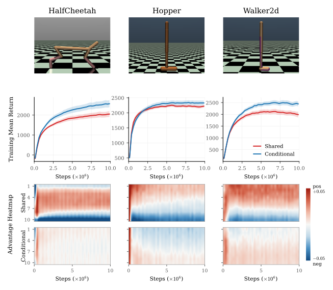
Mechanism checks and benchmark results

CartPole provides a controlled, end-to-end identification of value mismatch. MuJoCo asks whether the predicted advantage structure persists with continuous states, function approximation, and hidden dynamics variation. BipedalWalker and Procgen then test the practical value and scalability of critic conditioning across procedurally generated environments.

Critic architectures

Where the environment index enters

The actor is shared across environments and never receives z. Both critic designs retain a shared representation; they differ only in how the logged categorical index changes value prediction.

observation sactor network
shared across environmentspolicy π(a|s)z is not an actor input

(a)

FiLM critic

Feature modulation, one shared readout

observation sshared critic features h(s)

logged index zlookup c_zshared γ/β generators

\widetilde h_z=h(s)\odot(1+\gamma_z)+\beta_z

one shared value headV_FiLM(s,z)

(b)

Multihead critic

Shared features, indexed linear readout

observation sshared critic features h(s)

logged index zhead 1head zhead L

V_{\mathrm{mh}}(s,z)=w_z^\top h(s)+b_z

The index is training-only. At deployment the critic and z are discarded, leaving the same shared actor.

CartPole: controlled mechanism identification

CartPole dynamics and learned value comparison — The same state and action lead to different futures under two gravity values; environment-conditioned value predictions separate by gravity, while the shared critic's value prediction lies between them. Mean ± 1 s.d. over 20 seeds.

Two by five CartPole study comparing return, value loss, and advantages for shared, informative multihead, constant-index multihead, and per-level-bias critics under identical and heterogeneous gravity levels — Controlled identification of the CartPole mechanism, mean ± 1 standard error over 20 seeds. The top row uses two labeled levels with identical dynamics (g = 10); the bottom row uses g ∈ {10, 50}. Columns show mean return, value loss for levels 0 and 1, and the corresponding mean raw GAE advantages. With identical dynamics, all variants behave similarly. Under heterogeneous gravity, the multihead critic first pays a larger fitting cost on the hard level, then recenters its advantage and approaches a return of 200. Constant-index routing closely tracks the shared critic, whereas one learned scalar bias per level provides only a partial correction.

01 · Symptom

One value target leaves the hard level off center.

The shared critic keeps the hard level's mean raw GAE advantage negative while its return remains lower and more variable than the informative multihead critic.

02 · Transient fitting cost

Conditional values must first be learned.

The informative multihead critic initially incurs a larger hard-head loss and a deeper negative advantage shift while its level-specific readout fits the hard target.

03 · Re-centering

The benefit appears after the fitting transient subsides.

As the hard head catches up, its advantage returns toward zero first and the multihead policy reaches the highest return.

04 · Attribution

Useful level information, not extra parameters.

A constant-index multihead closely follows the shared critic. A learned scalar bias helps only partially, so a state-independent offset is insufficient in this setting.

From mechanism to continuous control

BipedalWalker terrain and return curves — Left: BipedalWalker test return on 100 unseen terrains and the 5× parameter control, mean ± 1 s.d. over 10 seeds. Right: MuJoCo with ten body-mass levels; training returns and raw GAE advantage means, averaged over 30 seeds.

MuJoCo returns and raw advantage heatmaps — Left: BipedalWalker test return on 100 unseen terrains and the 5× parameter control, mean ± 1 s.d. over 10 seeds. Right: MuJoCo with ten body-mass levels; training returns and raw GAE advantage means, averaged over 30 seeds.

Critic fitting

Conditioning is not a persistent fitting bottleneck.

The early multihead transient in compact CartPole does not recur systematically on the larger benchmarks. The initially higher BipedalWalker loss falls to a comparable level, FiLM remains below the shared critic through most of training on all three MuJoCo tasks, and both conditioned critics finish below the shared critic in 11 of 16 Procgen games. Each curve is measured on its method's own on-policy training stream, so it diagnoses optimization burden rather than value accuracy on a common distribution. Under that interpretation, the return gains are not accompanied by a systematic deterioration in critic fitting.

View value loss diagnostics

BipedalWalker uses 10 seeds; each MuJoCo task uses 30. Curves show mean ± 1 s.d., with a separate vertical scale in each panel.

All 16 Procgen games over 25M environment steps, mean ± 1 s.d. over 10 seeds; each panel uses its own vertical scale.

Application scale: Procgen

Procgen learning curves for eight games — Evaluation return on the 200 pinned training levels for eight Procgen games over 25M environment steps. Curves show mean ± 1 s.d. over 10 seeds.

**Held-out Procgen return on unseen levels.** Final checkpoints are evaluated for one episode on each of 600 held-out levels per game; entries are mean ± 1 s.d. over 10 training seeds. Bold marks the best unrounded mean in each row.
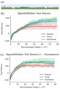
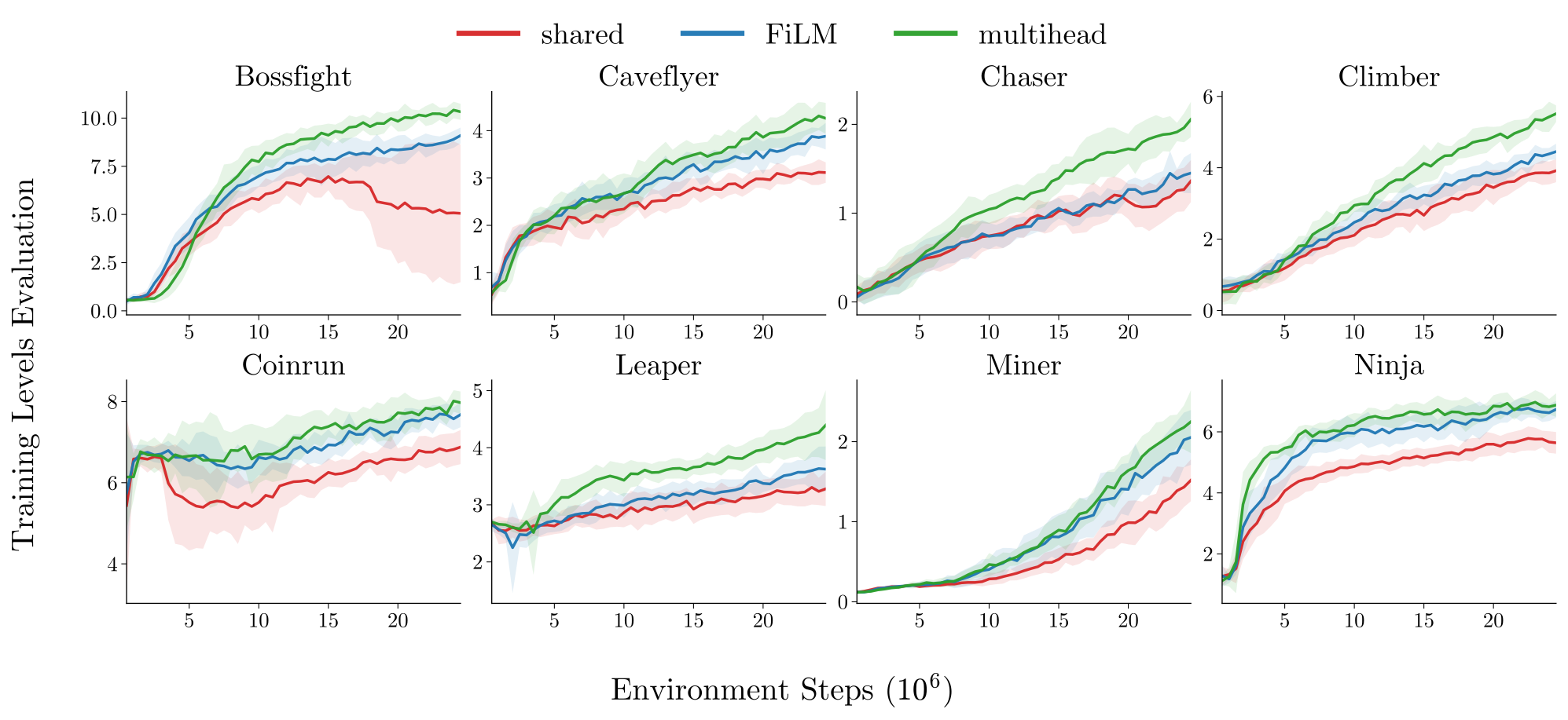
Game	Shared critic	FiLM critic	Multihead critic	Multihead + PopArt
Bigfish	1.87 ± 0.17	2.88 ± 0.57	2.99 ± 0.61	3.56 ± 1.27
Bossfight	4.44 ± 2.56	7.44 ± 0.51	8.97 ± 0.29	8.11 ± 0.82
Caveflyer	1.08 ± 0.16	1.90 ± 0.23	2.65 ± 0.43	1.87 ± 0.31
Chaser	0.95 ± 0.26	0.94 ± 0.19	1.32 ± 0.35	0.75 ± 0.17
Climber	1.40 ± 0.19	1.74 ± 0.27	2.75 ± 0.22	2.13 ± 0.27
Coinrun	5.76 ± 0.29	6.35 ± 0.28	6.80 ± 0.37	6.46 ± 0.29
Dodgeball	0.98 ± 0.05	0.91 ± 0.14	1.10 ± 0.20	1.32 ± 0.18
Fruitbot	7.39 ± 1.58	8.95 ± 0.70	8.14 ± 1.24	8.31 ± 1.01
Heist	0.24 ± 0.06	0.28 ± 0.05	0.20 ± 0.03	0.24 ± 0.06
Jumper	2.23 ± 0.13	2.36 ± 0.15	2.32 ± 0.12	2.35 ± 0.62
Leaper	2.81 ± 0.36	3.02 ± 0.24	3.25 ± 0.46	3.09 ± 0.28
Maze	1.23 ± 0.13	1.33 ± 0.13	1.49 ± 0.18	1.49 ± 0.15
Miner	0.53 ± 0.12	0.58 ± 0.08	0.80 ± 0.14	0.77 ± 0.13
Ninja	3.39 ± 0.21	3.98 ± 0.15	4.39 ± 0.29	4.10 ± 0.41
Plunder	2.37 ± 0.33	2.38 ± 0.18	2.28 ± 0.18	2.42 ± 0.29
Starpilot	7.96 ± 1.06	10.22 ± 1.11	13.10 ± 1.46	14.98 ± 2.35
Normalized held-out returns (%)	100.0 ± 19.8	121.2 ± 27.9	140.8 ± 47.1	133.3 ± 41.7

Additional conditioning-location ablations

BipedalWalker training return ablations — Training return.

BipedalWalker unseen test return ablations — Unseen test return.

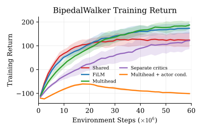
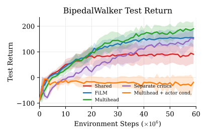
Separate critics learn more slowly, while supplying the environment index to the actor fails in this setting. These diagnostics isolate where conditioning enters; they are not part of the main intervention.

Scope

A mechanism and a minimal intervention

The formal results concern finite deterministic bandits with oracle baselines, a fixed environment mixture, and a common strict optimal arm. The deep-RL experiments test whether the mechanism-motivated intervention transfers beyond that abstraction.

The implementation uses finite, recurring environments with stable logged identities. The actor remains shared and does not receive the index in the proposed intervention.